Saturday, November 25, 2006

Processing vxstat to read into R

I got bored with my iostat data, and found some interesting looking vxstat logs to browse with the Cockcroft Headroom Plot. To get them into a regular format I wrote a short Awk script that is shown below. It skips the first record, adds a custom header and drops the time field into the first column.


# process vxstat file into regular csv format
BEGIN { skipping=1; printf("time,vol,reads,writes,breads,bwrites,tread,twrite\n"); }
NR < 4 {next} # skip header
NF > 0 && skipping==1 {next} # skip first record of totals since boot
NF == 0 {skipping=0}
NF == 5 {time=$0}
NF == 8 {printf("%s,%s,%s,%s,%s,%s,%s,%s\n",time,$2,$3,$4,$5,$6,$7,$8);}


It turns a file that looks like this:

OPERATIONS BLOCKS AVG TIME(ms)
TYP NAME READ WRITE READ WRITE READ WRITE

Mon May 01 19:00:01 2000
vol home 88159 346799 17990732 3680604 13.7 15.6
vol local 64308 103869 3848746 410899 6.0 22.0
vol orahome 80240 208372 18931823 886870 11.9 21.1
vol rootvol 336544 537741 21325442 8566302 4.8 323.1
vol swapvol 32857 339 4199304 58160 13.8 22.5
vol usr 396221 174834 11766646 2872832 3.5 547.6
vol var 316340 1688518 25138480 19275428 11.1 53.7

Mon May 01 19:00:31 2000
vol home 1 28 4 129 10.0 34.3
vol local 0 2 0 8 0.0 330.0
vol orahome 4 20 24 88 10.0 84.0
vol rootvol 0 80 0 720 0.0 9.4
vol swapvol 0 0 0 0 0.0 0.0
vol usr 0 1 0 16 0.0 20.0
vol var 4 235 54 2498 15.0 13.7

... and so on


into

% awk -f vx.awk < vxstat.out
time,vol,reads,writes,breads,bwrites,tread,twrite
Mon May 01 19:00:31 2000,home,1,28,4,129,10.0,34.3
Mon May 01 19:00:31 2000,local,0,2,0,8,0.0,330.0
Mon May 01 19:00:31 2000,orahome,4,20,24,88,10.0,84.0
Mon May 01 19:00:31 2000,rootvol,0,80,0,720,0.0,9.4
Mon May 01 19:00:31 2000,swapvol,0,0,0,0,0.0,0.0
Mon May 01 19:00:31 2000,usr,0,1,0,16,0.0,20.0
Mon May 01 19:00:31 2000,var,4,235,54,2498,15.0,13.7
... and so on


This can easily be read into R and plotted using


> vx <- read.csv("~/vxstat.csv", header=T)
> vxhome <- vx[vx$vol=="home",]
> chp(vxhome$reads,vxhome$treads)


One of the files I tried was quite long, half a million lines. It loaded into R in fifteen seconds, and the subsequent analysis operations didn't take too long. Try that with a spreadsheet... :-)

Slingbox for Xmas

What new toys can we get this Xmas? I already have the stuff I need. I'd like a phone with Wifi and 3G network speeds and a touch screen, but my Treo 650 is OK until something better comes along. I'm curious to see what Apple may come up with next year, in the much rumoured iPhone.

I've had a Tivo since 1999, and I'd like to be able to view the programs elsewhere in the house or further afield. The Slingbox does this, lets me control the Tivo remotely and stream the programs to a Windows or OSX laptop. The Slingbox AV was $179 list price on their web site, but I had a look on shopping.com and found it for sale from an out of state vendor for $140 with free shipping and no tax. So that's going to be the new toy this Xmas....

Thursday, November 23, 2006

Cockcroft Headroom Plot - Part 3 - Histogram Fixes

I found that I had some scaling issues with the histograms that needed fixing. Ultimately this made the code look a lot more complex, but it now deals with scaling the plot and the histogram with a fixed zero origin on both axes. I think its important to maintain the zero origin for a throughput vs. response time plot.

The tricky part is that the main plot is automatically oversized from its data range by a few percent, and the units used in the histogram are completely different. A histogram with 6 bars is scaled to have the bars at unit intervals and is 6 wide plus the width of the bars etc. After lots of trial and error, I made the main plot use the maximum bucket size of the histogram as its max value, and artificially offset the histograms by what looks like about the right amount. The plot below uses fixed data as a test. You can see that the first bar includes two points, thats due to the particular algorithm used by R. Some alternative histogram algorithms are available, but this one seems to be most appropriate to throughput/response time data.

> chp(5:10,5:10)


The updated code follows.

chp <- function(x,y,xl="Throughput",yl="Response",tl="Throughput Over Time",
ml="Cockcroft Headroom Plot") {
xhist <- hist(x,plot=FALSE)
yhist <- hist(y, plot=FALSE)
xbf <- xhist$breaks[1] # first
ybf <- yhist$breaks[1] # first
xbl <- xhist$breaks[length(xhist$breaks)] # last
ybl <- yhist$breaks[length(yhist$breaks)] # last
xcl <- length(xhist$counts) # count length
ycl <- length(yhist$counts) # count length
xrange <- c(0,xbl)
yrange <- c(0,ybl)
nf <- layout(matrix(c(2,4,1,3),2,2,byrow=TRUE), c(3,1), c(1,3), TRUE)
layout.show(nf)
par(mar=c(5,4,0,0))
plot(x, y, xlim=xrange, ylim=yrange, xlab=xl, ylab=yl)
par(mar=c(0,4,3,0))
barplot(xhist$counts, axes=FALSE,
xlim=c(xcl*0.03-xbf/((xbl-xbf)/(xcl-0.5)),xcl*0.97),
ylim=c(0, max(xhist$counts)), space=0, main=ml)
par(mar=c(5,0,0,1))
barplot(yhist$counts, axes=FALSE, xlim=c(0,max(yhist$counts)),
ylim=c(ycl*0.03-ybf/((ybl-ybf)/(ycl-0.5)),ycl*0.97),
space=0, horiz=TRUE)
par(mar=c(2.5,1.7,3,1))
plot(x, main=tl, cex.axis=0.8, cex.main=0.8, type="S")
}

Monday, November 20, 2006

Cockcroft Headroom Plot - Part 2 - R Version

I kept tweaking the code, and came up with a prettier version, that also has a small time series view of the throughput in the top right corner.


The code for this is

chp <- function(x,y,xl="Throughput",yl="Response",tl="Throughput Time Series", ml="Cockcroft Headroom Plot") {
xhist <- hist(x,plot=FALSE)
yhist <- hist(y, plot=FALSE)
xrange <- c(0,max(x))
yrange <- c(0,max(y))
nf <- layout(matrix(c(2,4,1,3),2,2,byrow=TRUE), c(3,1), c(1,3), TRUE)
layout.show(nf)
par(mar=c(5,4,0,0))
plot(x, y, xlim=xrange, ylim=yrange, xlab=xl, ylab=yl)
par(mar=c(0,4,3,0))
barplot(xhist$counts, axes=FALSE, ylim=c(0, max(xhist$counts)), space=0, main=ml)
par(mar=c(5,0,0,1))
barplot(yhist$counts, axes=FALSE, xlim=c(0,max(yhist$counts)), space=0, horiz=TRUE)
par(mar=c(2.5,1.5,3,1))
plot(x, main=tl, cex.axis=0.8, cex.main=0.8, type="S")
}


I also made a wrapper function that steps through the data over time in chunks.

> chp.step <- function(x, y, steps=10, secs=1.0) {
xl <- length(x)
step <- xl/steps
for(n in 0:(steps-1)) {
Sys.sleep(secs)
chp(x[(1+n*step):min((n+1)*step,xl)],y[(1+n*step):min((n+1)*step,xl)])
}
}


To run this smoothly on windows, I had to disable double buffering using

> options("windowsBuffered"=FALSE)

and close the graphics window so that a new one opens with the new option.

The data is displayed using the same calls as described in Part 1. The next step is to try some different data sets and work on detecting saturation automatically.

Sunday, November 19, 2006

The Cockcroft Headroom Plot - Part 1 - Introducing R

I've recently written a paper for CMG06 called "Utilization is Virtually Useless as a Metric!". Regular readers of this blog will recognize much of the content in that paper. The follow-on question is what to use instead? The answer I have is to plot response time vs. throughput, and I've been thinking about a very specific way to display this kind of plot. Since I'm feeling quite opinionated about this I'm going to call it a "Cockcroft Headroom Plot" and I'm going to try and construct it using various tools. I will blog my way through the development of this, and I welcome advice and comments along the way.

The starting point is a dataset to work with, and I found an old iostat log file that recorded a fairly busy disk at 15 minute intervals over a few days. This gives me 250 data points, which I fed into the R stats package to look at. I'll also have a go at making a spreadsheet version.

The iostat data file starts like this:
                    extended device statistics              
r/s w/s kr/s kw/s wait actv wsvc_t asvc_t %w %b device
14.8 78.4 183.0 2446.3 1.7 0.6 18.6 6.6 1 21 c1t5d0
0.0 0.0 0.0 0.0 0.0 0.0 0.0 5.0 0 0 c0t6d0
...

I want the second line as a header, so save it (my command line is actually on OSX, but could be Solaris, Linux or Cygwin on Windows)
% head -2 iostat.txt | tail -1 > header

I want the c1t5d0 disk, but don't want the first line, since its the average since boot, and want to add back the header
% grep c1t5d0 iostat.txt | tail +2 > tailer
% cat header tailer > c1t5.txt

Now I can import into R as a space delimited file with a header line. R doesn't allow "/" or "%" in names, so it rewrites the header to use dots instead. R is a script based tool with a command line and a very powerful vector/object based syntax. A "data frame" is a table of data object like a sheet in a spreadsheet, it has names for the rows and columns, and can be indexed.
> c1t5 <- read.delim("c1t5.txt",header=T,sep="")
> names(c1t5)
[1] "r.s" "w.s" "kr.s" "kw.s" "wait" "actv" "wsvc_t" "asvc_t" "X.w" "X.b" "device"

I only want to work with the first 250 data points so I subset the data frame by indexing the rows with an array (1:250) that selects the rows I want and leaving the column selector blank.
> io250 <- c1t5[1:250,]

The first thing to do is summarize the data, the output is too wide for the blog so I'll do it in chunks by selecting columns.

> summary(io250[,1:4])
r.s w.s kr.s kw.s
Min. : 1.80 Min. : 1.8 Min. : 13.5 Min. : 38.5
1st Qu.: 10.30 1st Qu.: 87.1 1st Qu.: 107.4 1st Qu.: 2191.7
Median : 18.90 Median :172.4 Median : 182.8 Median : 4279.4
Mean : 22.85 Mean :187.5 Mean : 290.1 Mean : 4448.5
3rd Qu.: 28.88 3rd Qu.:274.6 3rd Qu.: 287.4 3rd Qu.: 6746.6
Max. :130.90 Max. :508.8 Max. :4232.3 Max. :13713.1
> summary(io250[,5:8])
wait actv wsvc_t asvc_t
Min. : 0.000 Min. :0.0000 Min. : 0.000 Min. : 1.000
1st Qu.: 0.000 1st Qu.:0.3250 1st Qu.: 0.400 1st Qu.: 3.125
Median : 0.600 Median :0.8000 Median : 2.550 Median : 4.700
Mean : 1.048 Mean :0.9604 Mean : 5.152 Mean : 4.634
3rd Qu.: 1.300 3rd Qu.:1.5000 3rd Qu.: 6.350 3rd Qu.: 5.700
Max. :10.600 Max. :3.5000 Max. :88.900 Max. :15.100
> summary(io250[,9:10])
X.w X.b
Min. :0.000 Min. : 2.00
1st Qu.:0.000 1st Qu.:20.00
Median :1.000 Median :39.50
Mean :1.428 Mean :37.89
3rd Qu.:2.000 3rd Qu.:55.00
Max. :9.000 Max. :92.00


Looks like a nice busy disk, so lets plot everything against everything (pch=20 sets a solid dot plotting character)
> plot(io250[,1:10],pch=20)
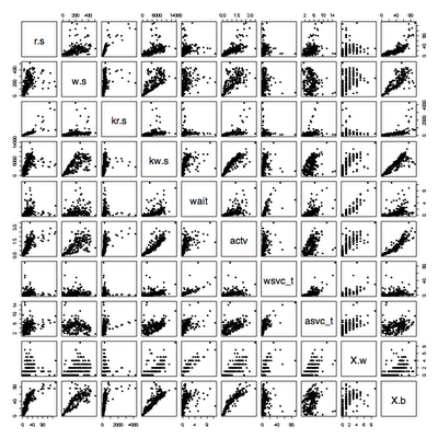
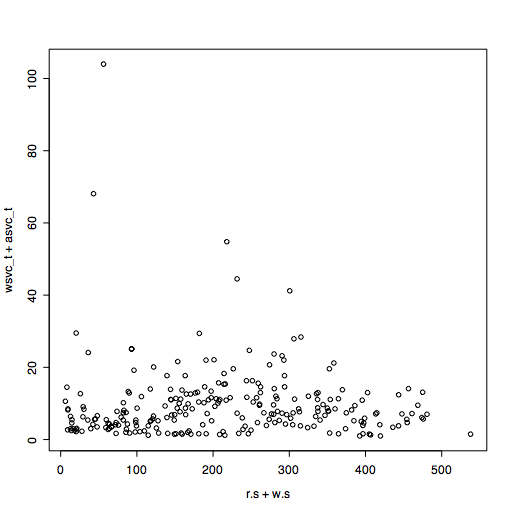
The throughput is either reads+writes or KB read+KB written, the response time is wsvc_t+asvc_t since iostat records time taken waiting to send to a disk as well as time spent actively waiting for a disk.

To save typing, I attach to the data frame so that the names are recognized directly.
> attach(io250)
> plot(r.s+w.s, wsvc_t+asvc_t)
This looks a bit scattered, because there is a mixture of average I/O sizes that varies during the time period. Lets look at throughput in KB/s instead.
> plot(kr.s+kw.s,wsvc_t+asvc_t)
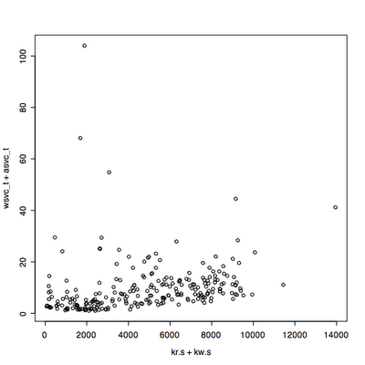
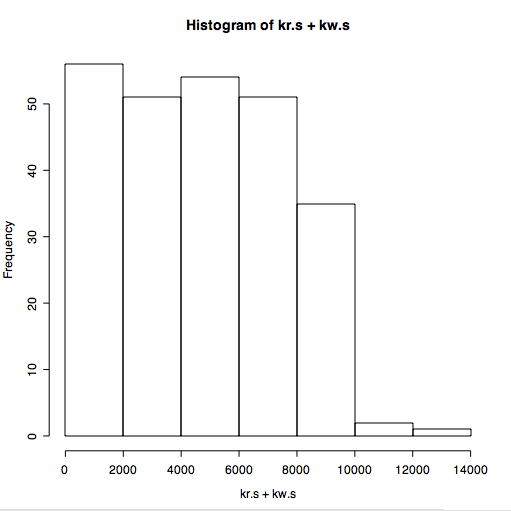
That looks promising, but its not clear what the distribution of throughput is over the range. We can look at this using a histogram.
> hist(kr.s+kw.s)

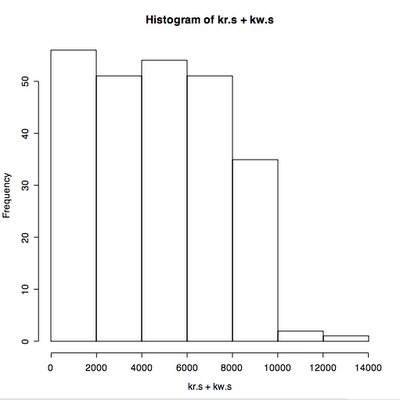
We can also look at the distribution of response times.
> hist(wsvc_t+asvc_t)
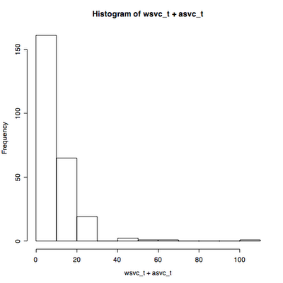
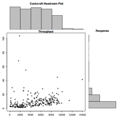
The starting point for the thing that I want to call a "Cockcroft Headroom Plot" is all three of these plots superimposed on each other. This means rotating the response time plot 90 degrees so that its axis lines up with the main plot. After looking around in the manual pages I eventually found an example that I could use as the basis for my plot. It needs some more cosmetic work but I defined a new function chp(throughput, response) shown below.

> chp <- function(x,y,xl="Throughput",yl="Response",ml="Cockcroft Headroom Plot") {
xhist <- hist(x,plot=FALSE)
yhist <- hist(y, plot=FALSE)
xrange <- c(0,max(x))
yrange <- c(0,max(y))
nf <- layout(matrix(c(2,0,1,3),2,2,byrow=TRUE), c(3,1), c(1,3), TRUE)
layout.show(nf)
par(mar=c(3,3,1.5,1.5))
plot(x, y, xlim=xrange, ylim=yrange, main=xl) par(mar=c(0,3,3,1))
barplot(xhist$counts, axes=FALSE, ylim=c(0, max(xhist$counts)), space=0, main=ml)
par(mar=c(3,0,1,1))
barplot(yhist$counts, axes=FALSE, xlim=c(0, max(yhist$counts)), space=0, main=yl, horiz=TRUE)
}

The result of running chp(kr.s+kw.s,wsvc_t+asvc_t)is close...


That's enough to get started.

ps3 Marketplace Research on eBay


Over at Data Mining there is some interesting info on ps3's.

However, there is no need to do manual scraping of
eBay, here is a screenshot from the marketplace research function
that is bundled with my eBay store subscription. For $2.99 for 2 days
access anyone can get at this.

http://pages.ebay.com/marketplace_research/

Skype on Solaris

http://blogs.sun.com/darren/entry/skype_1.3.0.53_on_solaris_via

Solaris has a Linux compatible subsystem called BrandZ for running Linux binaries that don't have Solaris builds (like Skype). Darren figured out how to get the Linux build of Skype to run on Opensolaris.

Thanks to Alec for pointing this out.


Saturday, November 11, 2006

10 Things to Know About Skype Ap2Ap Programming

I also posted this on the Skype Developer Wiki

The ap2ap capability is an interesting new network computing paradigm but it is not like a conventional network.
  1. end nodes are addressed by skype name, which addresses a person, not a computer

  2. people can login to skype multiple times, so addressable endpoints are not unique

  3. skype can go online/offline at will, so there is a concept of "presence" that needs to be managed

  4. you can only make ap2ap connections to your buddy list or people who you have chatted to "recently"

  5. both ends of an ap2ap connection have to choose a unique string used to identify their conversation or protocol

  6. if you quit and restart skype, the first login can persist for a while, so you can get multiple ap2ap connections from a single user, although the ghosts of your previous connections cannot respond to a message. I think is is because you connect to a different supernode each time, and the first one isn't sure if you have really gone away yet

  7. messages have to be sent as text, so binary objects have to be converted first using something like base64

  8. the network can behave differently each time you use it, and this non-determinism makes testing difficult

  9. relayed connections are limited to about 3KB/s, direct ones can run at several MB/s over a LAN

  10. Skype4Java is cross-platform, but the maximum message size is about 64KB on windows and 16KB on OSX/Linux, and there are several bugs and limitations in the older version of the API library that is used by Skype 2.0 and earlier releases. Use Skype 2.5 or later for the best performance and stability